Cosegregation

Cosegregation is the transmission to the next generation, of two or more genes in proximity on the same chromosome. Their closeness means that they are genetically linked. It may also represent an interaction estimation probability between any number of loci.

A. Nucleus, B. Nuclear Profile - Thin slice of Nucleus, C. Loci - Parts of a target gene found within the Nuclear Profile

Interaction probability is determined using specified parts of a target gene (loci) and a group of nuclear profiles (NPs). The picture to the right serves to provide visual aid as to how a slice (NP) is taken from the nucleus and loci are searched for within the NP. Cosegregation used within other mathematical models (SLICE and normalized linkage disequilibrium) assist in rendering 3-D visualizations as a smaller process of genome architecture mapping (GAM). These renderings help determine genomic density and radial position.

Articles Using Co-segregation Methodologies Title Description Complex multi-enhancer contacts captured by Genome Architecture Mapping (GAM). Co-segregation between a pair of loci helped in this study to quantify Normalized Linkage Disequilibrium. A simple method for cosegregation analysis to evaluate the pathogenicity of unclassified variants; BRCA1 and BRCA2 as an example. Using co-segregation analysis along with a multifactorial approach resulted in highly conclusive results when attempting to classify unclassified variants. Considerations in assessing germline variant pathogenicity using co-segregation analysis. This article found that utilizing Bayes factor co-segregation analysis, along with a strong penetrance model, will result with higher accuracy than meiosis counting.

History

Cosegregation in Genome architecture mapping (GAM) is another process being used to identify the compaction and adjacency of genomic windows. In a study from 2017, cosegregation was used to understand gene-expression-specific contacts in organizing the genome in mammalian nuclei in the larger process of GAM. The results of the study produced complex 3D structures that displayed interactions under certain regions of chromatin contacts and proved that GAM is a useful tool in the genome biologist's skill set that expands the ability to finely dissect 3D chromatin structures, cell types and valuable human samples. A study in 2021 "discovered extensive 'melting' of long genes when they are highly expressed and/or have high chromatin accessibility. The contacts most specific of neuron subtypes contain genes associated with specialized processes, such as addiction and synaptic plasticity, which harbour putative binding sites for neuronal transcription factors within accessible chromatin regions." Both of these studies used mice as models due to their anatomical, physiological, and genetic similarity to humans.

Some of the earliest known studies that have used cosegregation dates back to the early 1980s. Around this time, scientists were conducting experiments on vegetative organisms to see the if there are unique sequences of chloroplast DNA. The process of the experiment was to track the chloroplast gene in each generation by clustering the genes in nucleoids to reduce the number of segregated units. This study was done at the Duke University in the Zoology Department where Karen P. VanWinkle-Swift utilized Pedigree Diagrams to show how the traits and sequences were passed down from parent to child.

Usage

Cosegregation is best suited for cases where multiple factors' interactions are under consideration. It can show how different factors are linked and highlight their interactions and connections. For example, if a genetic disorder was identified as related to a certain gene, but is not always present when that gene is, then a cosegregation analysis could help identify other genes that interact with the suspect gene more often than normal. This could lead researchers to discover the combination of genes that manifest the genetic disorder. Cosegregation is being actively used in medical fields like cancer research. It can highlight the strongest connections between genes in cases where cancer develops. This is useful because there often isn't a single gene causing cancer. Rather, cancer can be caused by a multitude of gene combinations. Cosegregation helps to show links between genes that could be forming these combinations.

Examples of using cosegregation

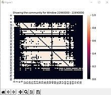
An example of an application using cosegregation would be finding the normalized linkage disequilibrium (NL) between two loci. Given a 2D dataset (row = genomic window slice, column = nuclear profile (NP)) a "1" was displayed if an NP existed in a window or a "0" otherwise. From this data, the NL could be found using the base $linkage$ disequilibrium and its theorized maximum ($dmax$). The amount of NPs present in loci (genomic windows) $A$ and $B$, is then used to find the $detectionfrequencies$, $fa$ and $fb$ and the co-segregation which is, $fab$. after the NL is found between two loci, it was then placed into another dataset to be visualized and then analyzed to determine how interconnected a loci is. This example was executed using python for computation and visualization of the given data and results and in finding the NL. Using the NL further analysis can be done to place the windows into "communities". To showcase this a graph to the right will show the community of one of the windows with the highest centrality which uses the average of the window's NLs.

Displays the communities for a specific loci using centrality

A sample of the 2D dataset that was used for the application of the cosegregation example.

Formulas for the example above Calculations Formulas Detection Frequency $\left({\frac {A}{N}}\right)$ or $fa$ Linkage $\left({\frac {AB}{N}}\right)-(\left({\frac {A}{N}}\right)*\left({\frac {B}{N}}\right))$ Linkage maximum (dmax) :$$dmax={\begin{cases}min(fafb,(1-fa)(1-fb)),&{\text{when }}linkage<0\\min(fb(1-fa),fa(1-fb)),&{\text{when }}linkage\geq 0.\end{cases}}$$ Normalized Linkage (NL) $NL=linkage/dmax$

Formula

pseudo-code showcasing the implementation of co-segregation in data science.

Formula for finding co-segregation given a GAM table showing if a loci is present in a slice of a genomic region Formula Variables $\left({\frac {AB}{N}}\right)$ or $fAB$ Variables "A" and "B" are the total number of nuclear profiles (NP) present in a given a detected genomic region slice, "N" is the total number of NPs and FAB is the frequency of A and B

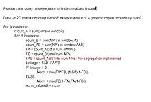
This formula can be easily programmed into code as seen in the pseudo-code in the figure to the right. The code was written to satisfy the Example described above.

Advantages

Given a large dataset of nuclear profiles, cosegregation is easily scalable given its simplistic mathematical formulas. The larger the data set that is provided, the more accurate the following equations will be. As depicted in the photo below, the amount of data being added to the equation merely adds linear time adjustments to the original equation.

How adding more NPs to dataset affects cosegregation equation.

Fortunately, not only is it able to scale dataset sizes well, it is able to take as many loci of focus that are required to determine the interaction probability. Provided that adding each loci adds a single computation to the equation, a linear time complexity is the result. The picture below shows how the amount of loci affects the detection frequency equation.

Adding loci affects the cosegregation equation in a linear time complexity.

Finally, the numerical value that results can assist in drawing multiple conclusions including radial position, compaction, and the most influential contacts.

Limitations

This co-segregation heat map of genetic windows has not been normalized, the pattern is much less clear and the data is not as meaningful compared to the normalized version.

This co-segregation heat map of genetic windows has been normalized, the pattern is much more clear and that data can more easily and accurately be interpreted.

Effective cosegregation analysis depends largely on having a strong supporting dataset because even small inaccuracies can be compounded by cosegregation. A complete understanding of the material is necessary as cosegregation only provides connections between datapoints. The interpretation of those connections must be done through another method. For example, locus cosegregation can give a score of genes that commonly interact with each other, but no matter how strong those relationships are, the results of quantitative cosegregation can seem to support either a correlated, anti-correlated or independent relationships. It is important to be aware of this and follow up cosegregation analysis with another form of analysis, such as normalized linkage disequilibrium to correct for the compounding effect cosegregation can have on negligible variations in the detection frequency of the data.

For example, imagine a simple form of cancer that is trigged by a small number of genes. Here we are examining a suspect gene and three other genes that are suspected to be involved in the processes. This chart shows a hypothetical data set of 10 people and their cancer status as well as if they possess the four genes of interest. Looking at the graph, there is a clear connection between the suspect gene and Gene A. There is also a less obvious interaction between the suspect gene and Gene C that only takes place when Gene B is absent. It is entirely possible that co-segregation would have a hard time determining that relationship. Gene B is commonly present with Gene A and that combination does result in cancer. In a real data set with hundreds or even thousands of genes being examined, one could erroneously conclude that Gene B contributes to the cancer when, in reality it does not and can actually prevent it.

Another limitation of this technique is that many mapping tools measure not only specific physical interactions between genes but also random contacts, the latter being much more common between genes with smaller linear genomic distance this could lead to inflated co-segregation scores. GAM has helped to resolve this issue because in GAM the detection of genomic windows is independent of any interactions with other regions. This allows for an expected interaction value to be calculated and combining this with the co-segregation results to filter out the noise of random connections this will provide a cleaner result.

Visualizations

Matrices

Matrices are a rectangular structured array of numbers (entries) where the entries can be summed, subtracted, multiplied, and divided using the standard math operations. In the case of co-segregation, Graph theory is used to see if a variable shares an edge or vertex with another variable on a network of nodes. Graph theory is the mathematical study of objects using pairwise relations that is shown through connected nodes called vertices that are connected to other nodes by edges.

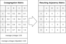
The image above depicts the conversion from a cosegregation matrix to an adjacency matrix is one use of a matrix in genome architecture mapping where scientists are using cryosectioning to find colocalization between DNA regions, genomes, and/or alleles. In that example, cosegregation is being used to describe the linkage of data to each other in terms of the distance between specific windows in a genome. The values in the cosegregation matrix were found using the formula above. Comparing windows A and B, the formula seeks to find the intersection of Nuclear Profiles between the respective windows. The genomic windows would be the nodes and the adjacency graph is the matrix depiction of the edges connecting each node.

Heat maps

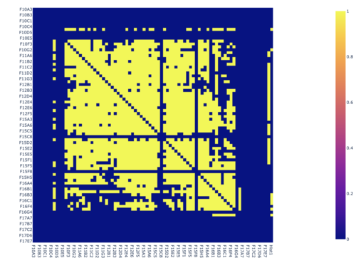
A heat map is a visual representation of a matrix of m × n that can show different phenomenons on a two-dimensional scale. Heat maps have a range of color intensities based on the values and scale given from the data. Coding-wise, heat maps can be created using libraries such as plotly.express in Python. Using co-segregation, heat maps are used to visualize a matrix that contains values of either 1 or 0 to visualize the commonalities between 2 or more variables. "The primary benefit of using heat maps is that they make otherwise dull or impenetrable data understandable. Many people understand heat maps intuitively, without even needing to be told that those warmer colors indicate a denser focus of interactions."

In the limitation section, there are two heat maps (also put below for easy viewing) shown depicting the difference between normalized and un-normalized data. Showing the difference in the graphs would help the researcher identify different patterns based on the intensity of the color gradients as well as the clustering of data points. Cosegregation results as seen above can have different forms and visualizing them in heat maps can aid researchers in understanding which genomes are connected similar to matrices.

One limitation to heat maps are that some software does not allow the use of locating specific points on the graph, especially if there are many variables. There are coding libraries such as plotly.express that can create interactive heat maps where the programmer can hover over specified points on a graph and read the exact dependent variable's value. Another limitation is that heat maps do not represent real-time data. Since heat maps work by aggregating data over time, it does not show recent changes in behavior compared to the more dominant patterns already present.

References

[edit]- ^ "Cosegregation". cancer.gov. Retrieved 4 May 2023.
- ^ Wrighton, Katharine H. (May 2017). "Zooming in on nuclear organization". Nature Reviews Molecular Cell Biology. 18 (5): 275. doi:10.1038/nrm.2017.28. PMID 28327555. S2CID 3453730.
- ^ a b c d e f g Beagrie, Robert A.; Scialdone, Antonio; Schueler, Markus; Kraemer, Dorothee C. A.; Chotalia, Mita; Xie, Sheila Q.; Barbieri, Mariano; de Santiago, Inês; Lavitas, Liron-Mark; Branco, Miguel R.; Fraser, James; Dostie, Josée; Game, Laurence; Dillon, Niall; Edwards, Paul A. W.; Nicodemi, Mario; Pombo, Ana (March 2017). "Complex multi-enhancer contacts captured by genome architecture mapping". Nature. 543 (7646): 519–524. Bibcode:2017Natur.543..519B. doi:10.1038/nature21411. PMC 5366070. PMID 28273065.
- ^ Mohammadi, Leila; Vreeswijk, Maaike P; Oldenburg, Rogier; van den Ouweland, Ans; Oosterwijk, Jan C; van der Hout, Annemarie H; Hoogerbrugge, Nicoline; Ligtenberg, Marjolijn; Ausems, Margreet G; van der Luijt, Rob B; Dommering, Charlotte J; Gille, Johan J; Verhoef, Senno; Hogervorst, Frans B; van Os, Theo A; Gómez García, Encarna; Blok, Marinus J; Wijnen, Juul T; Helmer, Quinta; Devilee, Peter; van Asperen, Christi J; van Houwelingen, Hans C (29 June 2009). "A simple method for co-segregation analysis to evaluate the pathogenicity of unclassified variants; BRCA1 and BRCA2 as an example". BMC Cancer. 9: 211. doi:10.1186/1471-2407-9-211. PMC 2714556. PMID 19563646.
- ^ Belman, Sophie; Parsons, Michael T.; Spurdle, Amanda B.; Goldgar, David E.; Feng, Bing-Jian (December 2020). "Considerations in assessing germline variant pathogenicity using cosegregation analysis". Genetics in Medicine. 22 (12): 2052–2059. doi:10.1038/s41436-020-0920-4. PMID 32773770. S2CID 221084291.
- ^ Winick-Ng, Warren; Kukalev, Alexander; Harabula, Izabela; Zea-Redondo, Luna; Szabó, Dominik; Meijer, Mandy; Serebreni, Leonid; Zhang, Yingnan; Bianco, Simona; Chiariello, Andrea M.; Irastorza-Azcarate, Ibai; Thieme, Christoph J.; Sparks, Thomas M.; Carvalho, Sílvia; Fiorillo, Luca; Musella, Francesco; Irani, Ehsan; Torlai Triglia, Elena; Kolodziejczyk, Aleksandra A.; Abentung, Andreas; Apostolova, Galina; Paul, Eleanor J.; Franke, Vedran; Kempfer, Rieke; Akalin, Altuna; Teichmann, Sarah A.; Dechant, Georg; Ungless, Mark A.; Nicodemi, Mario; Welch, Lonnie; Castelo-Branco, Gonçalo; Pombo, Ana (November 2021). "Cell-type specialization is encoded by specific chromatin topologies". Nature. 599 (7886): 684–691. Bibcode:2021Natur.599..684W. doi:10.1038/s41586-021-04081-2. PMC 8612935. PMID 34789882.
- ^ Bryda, Elizabeth C (May 2013). "The Mighty Mouse: the impact of rodents on advances in biomedical research". Missouri Medicine. 110 (3): 207–211. PMC 3987984. PMID 23829104.
- ^ VanWinkle-Swift, Karen P. (February 1980). "A model for the rapid vegetative segregation of multiple chloroplast genomes in Chlamydomonas: Assumptions and predictions of the model". Current Genetics. 1 (2): 113–125. doi:10.1007/BF00446957. PMID 24190835. S2CID 19184456.
- ^ a b "Heat Maps: Types & Benefits".