Fisher transformation

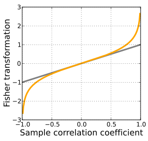
In statistics, the Fisher transformation (or Fisher z-transformation) of a Pearson correlation coefficient is its inverse hyperbolic tangent (artanh). When the sample correlation coefficient r is near 1 or -1, its distribution is highly skewed, which makes it difficult to estimate confidence intervals and apply tests of significance for the population correlation coefficient ρ.[1][2][3] The Fisher transformation solves this problem by yielding a variable whose distribution is approximately normally distributed, with a variance that is stable over different values of r.
Definition
[edit]Given a set of N bivariate sample pairs (Xi, Yi), i = 1, ..., N, the sample correlation coefficient r is given by
Here stands for the covariance between the variables and and stands for the standard deviation of the respective variable. Fisher's z-transformation of r is defined as
where "ln" is the natural logarithm function and "artanh" is the inverse hyperbolic tangent function.
If (X, Y) has a bivariate normal distribution with correlation ρ and the pairs (Xi, Yi) are independent and identically distributed, then z is approximately normally distributed with mean
and a standard deviation which does not depend on the value of the correlation rho (i.e., a Variance-stabilizing transformation)
where N is the sample size, and ρ is the true correlation coefficient.
This transformation, and its inverse
can be used to construct a large-sample confidence interval for r using standard normal theory and derivations. See also application to partial correlation.
Derivation
[edit]This article may require cleanup to meet Wikipedia's quality standards. The specific problem is: the steps of the derivation are not laid out completely. (July 2021) |

Hotelling gives a concise derivation of the Fisher transformation.[4]
To derive the Fisher transformation, one starts by considering an arbitrary increasing, twice-differentiable function of , say . Finding the first term in the large- expansion of the corresponding skewness results[5] in
Setting and solving the corresponding differential equation for yields the inverse hyperbolic tangent function.
Similarly expanding the mean m and variance v of , one gets
- m =
and
- v =
respectively.
The extra terms are not part of the usual Fisher transformation. For large values of and small values of they represent a large improvement of accuracy at minimal cost, although they greatly complicate the computation of the inverse – a closed-form expression is not available. The near-constant variance of the transformation is the result of removing its skewness – the actual improvement is achieved by the latter, not by the extra terms. Including the extra terms, i.e., computing (z-m)/v1/2, yields:
which has, to an excellent approximation, a standard normal distribution.[6]

Application
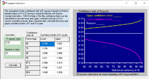
[edit]The application of Fisher's transformation can be enhanced using a software calculator as shown in the figure. Assuming that the r-squared value found is 0.80, that there are 30 data [clarification needed], and accepting a 90% confidence interval, the r-squared value in another random sample from the same population may range from 0.656 to 0.888. When r-squared is outside this range, the population is considered to be different.
Discussion
[edit]The Fisher transformation is an approximate variance-stabilizing transformation for r when X and Y follow a bivariate normal distribution. This means that the variance of z is approximately constant for all values of the population correlation coefficient ρ. Without the Fisher transformation, the variance of r grows smaller as |ρ| gets closer to 1. Since the Fisher transformation is approximately the identity function when |r| < 1/2, it is sometimes useful to remember that the variance of r is well approximated by 1/N as long as |ρ| is not too large and N is not too small. This is related to the fact that the asymptotic variance of r is 1 for bivariate normal data.
The behavior of this transform has been extensively studied since Fisher introduced it in 1915. Fisher himself found the exact distribution of z for data from a bivariate normal distribution in 1921; Gayen in 1951[8] determined the exact distribution of z for data from a bivariate Type A Edgeworth distribution. Hotelling in 1953 calculated the Taylor series expressions for the moments of z and several related statistics[9] and Hawkins in 1989 discovered the asymptotic distribution of z for data from a distribution with bounded fourth moments.[10]
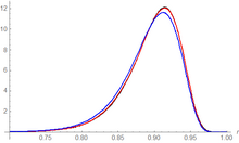
An alternative to the Fisher transformation is to use the exact confidence distribution density for ρ given by[11][12] where is the Gaussian hypergeometric function and .
Other uses
[edit]While the Fisher transformation is mainly associated with the Pearson product-moment correlation coefficient for bivariate normal observations, it can also be applied to Spearman's rank correlation coefficient in more general cases.[13] A similar result for the asymptotic distribution applies, but with a minor adjustment factor: see the cited article for details.
See also
[edit]- Data transformation (statistics)
- Meta-analysis (this transformation is used in meta analysis for stabilizing the variance)
- Partial correlation
- Pearson correlation coefficient § Inference
References
[edit]- ^ Fisher, R. A. (1915). "Frequency distribution of the values of the correlation coefficient in samples of an indefinitely large population". Biometrika. 10 (4): 507–521. doi:10.2307/2331838. hdl:2440/15166. JSTOR 2331838.
- ^ Fisher, R. A. (1921). "On the 'probable error' of a coefficient of correlation deduced from a small sample" (PDF). Metron. 1: 3–32.
- ^ Rick Wicklin. Fisher's transformation of the correlation coefficient. September 20, 2017. https://blogs.sas.com/content/iml/2017/09/20/fishers-transformation-correlation.html. Accessed Feb 15,2022.
- ^ Hotelling, Harold (1953). "New Light on the Correlation Coefficient and its Transforms". Journal of the Royal Statistical Society, Series B (Methodological). 15 (2): 193–225. doi:10.1111/j.2517-6161.1953.tb00135.x. ISSN 0035-9246.
- ^ Winterbottom, Alan (1979). "A Note on the Derivation of Fisher's Transformation of the Correlation Coefficient". The American Statistician. 33 (3): 142–143. doi:10.2307/2683819. ISSN 0003-1305. JSTOR 2683819.
- ^ Vrbik, Jan (December 2005). "Population moments of sampling distributions". Computational Statistics. 20 (4): 611–621. doi:10.1007/BF02741318. S2CID 120592303.
- ^ r-squared calculator
- ^ Gayen, A. K. (1951). "The Frequency Distribution of the Product-Moment Correlation Coefficient in Random Samples of Any Size Drawn from Non-Normal Universes". Biometrika. 38 (1/2): 219–247. doi:10.1093/biomet/38.1-2.219. JSTOR 2332329.
- ^ Hotelling, H (1953). "New light on the correlation coefficient and its transforms". Journal of the Royal Statistical Society, Series B. 15 (2): 193–225. JSTOR 2983768.
- ^ Hawkins, D. L. (1989). "Using U statistics to derive the asymptotic distribution of Fisher's Z statistic". The American Statistician. 43 (4): 235–237. doi:10.2307/2685369. JSTOR 2685369.
- ^ Taraldsen, Gunnar (2021). "The Confidence Density for Correlation". Sankhya A. doi:10.1007/s13171-021-00267-y. hdl:11250/3133125. ISSN 0976-8378. S2CID 244594067.
- ^ Taraldsen, Gunnar (2020). "Confidence in Correlation". doi:10.13140/RG.2.2.23673.49769.
{{cite journal}}: Cite journal requires|journal=(help) - ^ Zar, Jerrold H. (2005). "Spearman Rank Correlation: Overview". Encyclopedia of Biostatistics. doi:10.1002/9781118445112.stat05964. ISBN 9781118445112.


