Jump to content

File:Schwarz triangle function.svg

Page contents not supported in other languages.
This is a file from the Wikimedia Commons
From Wikipedia, the free encyclopedia

Original file (SVG file, nominally 619 × 601 pixels, file size: 222 KB)

Summary

 
The SVG code is valid.
 
This plot was created with Matplotlib.
Description
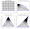
English: Plots of the Schwarz triangle function for various parameters.
  • Upper left: Untransformed upper half-plane
  • Upper right: Transformation of the upper half-plane by the Schwarz triangle function with α = 1/2, β = 1/2, γ = 1/3
  • Bottom left: Transformation of the upper half-plane by the Schwarz triangle function with α = β = γ = 1/3
  • Bottom right: Transformation of the upper half-plane by the Schwarz triangle function with α = 1/4, β = 1/10, γ = 1/3
Date
Source Own work
Author Apocheir
Source code
InfoField

Python code

Python code
import numpy as np
from scipy.special import hyp2f1, gamma
import matplotlib.pyplot as plt


def schwarz_sp(alpha, beta, gam):
    """Values of the Schwarz triangle map at 1 and infinity.
    Args:
        alpha, beta, gamma: Equal to pi times an angle of the triangle.
    Returns:
        s1: Value of the Schwarz triangle map at z=1.
        sinf: Value of the Schwarz triangle map at z=infinity.
        a, b, c, ap, bp, cp: Parameters to the hypergeometric functions.
    """
    a = (1 - alpha - beta - gam)/2
    b = (1 - alpha + beta - gam)/2
    c = 1 - alpha
    ap = (1 + alpha - beta - gam)/2  # a - c + 1
    bp = (1 + alpha + beta - gam)/2  # b - c + 1
    cp = 1 + alpha  # 2-c

    palpha = np.pi*alpha
    gfact = gamma(2-c)/(gamma(1-a)*gamma(c))
    s1 = gamma(c-a)*gamma(c-b)/gamma(1-b)*gfact
    sinf = np.exp(1j*palpha)*gamma(b)*gamma(c-a)*gfact/gamma(b-c+1)
    return s1, sinf, a, b, c, ap, bp, cp


def schwarz(alpha, beta, gam, z):
    s1, sinf, a, b, c, ap, bp, cp = schwarz_sp(alpha, beta, gam)
    result = z**alpha*hyp2f1(ap, bp, cp, z)/hyp2f1(a, b, c, z)
    result[np.isinf(z)] = sinf
    return result


n = 20
x = np.linspace(-n, n, 20*n+1)
y = np.arange(1, 2*n + 1)[:, np.newaxis]
grid_hor = (x + 1j*y).T
x = np.arange(-n, n+1)
y = np.linspace(0, 2*n, 20*n+1)[:, np.newaxis]
grid_vert = x + 1j*y
grid = np.concatenate([grid_hor, grid_vert], axis=1)
# the edges opposite angles beta and gamma are just straight lines, 
# so we can skimp on the points on those line [-inf to 1]
# and concentrate on the edge opposite alpha [1 to inf].
# spacing is chosen arbitrary to make it look smooth
boundary = np.concatenate([np.linspace(0, 1)**10 + 1,
                           np.logspace(1, 10, base=2),
                           [np.inf, -3, 0, 1]]) + 0j

# to fill in the part near s(inf) where the gridlines 
# become so close together that it just turns black
cap = np.concatenate([np.logspace(np.log2(n), 10, base=2),
                      [np.inf, -n]]) + 0j

fig, axes = plt.subplots(nrows=2, ncols=2, figsize=(8, 8))
for ax in axes.flat:
    ax.axis('equal')
ax = axes[0, 0]
ax.set_title('Upper half-plane')
ax.plot(grid.real, grid.imag, color='k')
ax.plot(boundary.real, boundary.imag, color='b')
ax.fill([-10, 10, 10, -10], [0, 0, 10, 10], color='lightgrey')
ax.set_xlim(-2, 2)
ax.set_ylim(-1, 4)

params = [(1/2, 1/2, 1/3),
          (1/3, 1/3, 1/3),
          (1/4, 1/10, 1/3)]
titles = ['α = 1/2, β = 1/2, γ = 1/3',
          'α = β = γ = 1/3',
          'α = 1/4, β = 1/10, γ = 1/3']
for ax, a, t in zip([axes[0, 1], axes[1, 0], axes[1, 1]], params, titles):
    g = schwarz(a[0], a[1], a[2], grid)
    b = schwarz(a[0], a[1], a[2], boundary)
    ax.plot(g.real, g.imag, color='k')
    ax.plot(b.real, b.imag, color='b', zorder=10)
    ax.fill(b.real, b.imag, color='lightgrey')
    c = schwarz(a[0], a[1], a[2], cap)
    ax.fill(c.real, c.imag, color='k')
    ax.set_title(t)

fig.savefig('schwarz triangle function.svg', bbox_inches='tight')

Licensing

I, the copyright holder of this work, hereby publish it under the following license:
Creative Commons CC-Zero This file is made available under the Creative Commons CC0 1.0 Universal Public Domain Dedication.
The person who associated a work with this deed has dedicated the work to the public domain by waiving all of their rights to the work worldwide under copyright law, including all related and neighboring rights, to the extent allowed by law. You can copy, modify, distribute and perform the work, even for commercial purposes, all without asking permission.

Captions

Plots of the Schwarz triangle function

Items portrayed in this file

depicts

16 August 2022

image/svg+xml

File history

Click on a date/time to view the file as it appeared at that time.

Date/TimeThumbnailDimensionsUserComment
current01:02, 18 August 2022Thumbnail for version as of 01:02, 18 August 2022619 × 601 (222 KB)Apocheirtitles, more distinct choice of parameters
02:28, 17 August 2022Thumbnail for version as of 02:28, 17 August 2022615 × 601 (226 KB)ApocheirUploaded own work with UploadWizard

The following page uses this file:

Metadata