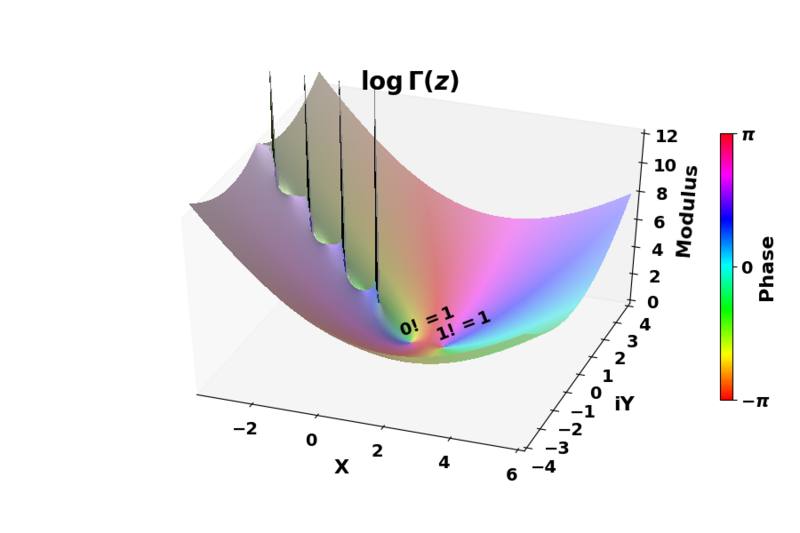
File:LogGamma Analytic Function.png
Page contents not supported in other languages.
Tools
Actions
General
In other projects
Appearance

Size of this preview: 800 × 533 pixels. Other resolutions: 320 × 213 pixels | 640 × 427 pixels.
Original file (900 × 600 pixels, file size: 108 KB, MIME type: image/png)
| This is a file from the Wikimedia Commons. Information from its description page there is shown below. Commons is a freely licensed media file repository. You can help. |
Summary
| DescriptionLogGamma Analytic Function.png |
English: Logarithmic Gamma Function Modulus and Phase; the analytic log-Gamma function  |
| Date | |
| Source |
Own work This plot was created with Matplotlib. |
| Author | stsmith |
Licensing
I, the copyright holder of this work, hereby publish it under the following license:
This file is licensed under the Creative Commons Attribution-Share Alike 4.0 International license.
- You are free:
- to share – to copy, distribute and transmit the work
- to remix – to adapt the work
- Under the following conditions:
- attribution – You must give appropriate credit, provide a link to the license, and indicate if changes were made. You may do so in any reasonable manner, but not in any way that suggests the licensor endorses you or your use.
- share alike – If you remix, transform, or build upon the material, you must distribute your contributions under the same or compatible license as the original.
Python Code
import matplotlib as mpl
import matplotlib.pyplot as plt
from matplotlib import cm
from mpl_toolkits.mplot3d import Axes3D
import numpy as np
import scipy.special as sps

# Import lighting object for shading surface plots.
from matplotlib.colors import LightSource

# Legible plot style defaults
# http://matplotlib.org/api/matplotlib_configuration_api.html
# http://matplotlib.org/users/customizing.html
mpl.rcParams['figure.figsize'] = (10.0, 5.0)
mpl.rc('font',**{'family': 'sans-serif', 'weight': 'bold', 'size': 14})
mpl.rc('axes',**{'titlesize': 20, 'titleweight': 'bold', 'labelsize': 16, 'labelweight': 'bold'})
mpl.rc('legend',**{'fontsize': 14})
mpl.rc('figure',**{'titlesize': 16, 'titleweight': 'bold'})
mpl.rc('lines',**{'linewidth': 2.5, 'markersize': 18, 'markeredgewidth': 0})
mpl.rc('mathtext',**{'fontset': 'custom', 'rm': 'sans:bold', 'bf': 'sans:bold', 'it': 'sans:italic', 'sf': 'sans:bold', 'default': 'it'})
# plt.rc('text',usetex=False) # [default] usetex should be False
mpl.rcParams['text.latex.preamble'] = [r'\usepackage{amsmath,sfmath} \boldmath']

realmin = np.finfo(np.double).tiny

# Define grid of points.
xpoints = np.linspace(-3.5, 6, int(np.round((6+3.5)*20))+1)
ypoints = np.linspace(-4, 4, (4+4)*20+1)
X, Y = np.meshgrid(xpoints, ypoints)
# n.b. np.gammaln, np.log(sps.gamma(X+Y*1j)) branch cuts are messed up
# e.g. xf = scipy.optimize.minimize(lambda x: np.abs(np.log(sps.gamma(x[0]+x[1]*1j))), np.array([4.,4.]), method='Nelder-Mead', tol=1.e-12)
F = sps.loggamma(X+Y*1j)
M = np.abs(F)
# n.b. this is phase of -log(gamma(z)), not log(gamma(z))
P = np.arctan2(-F.imag,-F.real)
nanscale = 1.33
M = np.where(np.isnan(M),nanscale*np.nanmax(M),M)
P = np.where(np.isnan(P),0.,P)

# Create an hsv array
H = (P+np.pi)/(2*np.pi)
S = np.ones_like(H)
V = 1.-(M-M.min())/(M.max()-M.min())

# Set view parameters for all subplots.
azimuth = 290
altitude = 41
# Create empty figure.
fig = plt.figure(figsize=(9,6))

# n.b. 1-hsv colors the colors the phase of -log(gamma(z)) correctly w.r.t. hsv cmap
facecolors = 1.-mpl.colors.hsv_to_rgb(np.dstack((H,S,V)))
f = 0.25
facecolors = f + (1-f)*facecolors

# light = LightSource(azimuth+20, altitude-10)
light = LightSource(120, 20)
illuminated_surface = light.shade_rgb(facecolors, M)

# Create a subplot with 3d plotting capabilities.
# This command will fail if Axes3D was not imported.
ax = fig.add_subplot(111, projection='3d')
ax.view_init(altitude, azimuth)
ax.plot_surface(X, Y, M, rstride=1, cstride=1, linewidth=0,
                antialiased=False, facecolors=illuminated_surface, shade=True)
plt.xlabel('X',labelpad=10)
plt.ylabel('iY',labelpad=10)
plt.title('$\log\,\Gamma(z)$')
ax.set_zlabel('Modulus',labelpad=5)
ax.set_xlim([xpoints.min(), xpoints.max()])
ax.set_ylim([ypoints.min(), ypoints.max()])
ax.set_zlim([0, np.floor(M.max()/nanscale/2)*2])
ax.grid(False)

ax.text(0.5, 0.25, 1.5, r'$0! = 1$', (1,0.5,0.5))
ax.text(1.5, 0.5, 1.25, r'$1! = 1$', (1,0.5,0.5))

cax = fig.add_axes([0.9, 0.25, 0.015, 0.5])
cb = mpl.colorbar.ColorbarBase(cax, cmap=plt.cm.hsv, spacing='proportional', ticks=[0, 0.5, 1])
cb.ax.set_yticklabels(['$-\pi$', '$0$', '$\pi$'])
cb.set_label('Phase',labelpad=-10)
plt.savefig('./loggamma.png')
Captions
Add a one-line explanation of what this file represents
Items portrayed in this file
depicts
some value
26 April 2017
File history
Click on a date/time to view the file as it appeared at that time.
| Date/Time | Thumbnail | Dimensions | User | Comment | |
|---|---|---|---|---|---|
| current | 13:51, 26 April 2017 |  | 900 × 600 (108 KB) | Stsmith | User created page with UploadWizard |
File usage
The following page uses this file:
Global file usage
The following other wikis use this file:
- Usage on ca.wikipedia.org
- Usage on fr.wikipedia.org
Metadata
This file contains additional information, probably added from the digital camera or scanner used to create or digitize it.
If the file has been modified from its original state, some details may not fully reflect the modified file.
| Horizontal resolution | 39.37 dpc |
|---|---|
| Vertical resolution | 39.37 dpc |
Retrieved from "https://en.wikipedia.org/wiki/File:LogGamma_Analytic_Function.png"
